This post is aimed for a little bit advanced reader, though those who have at least any interest towards theoretical physics will find it interesting and rather useful. Here I’m going to introduce an interesting physics apparatus called Penrose diagrams, which is intensively used in general theory of relativity and especially in black hole thermodynamics. As I didn’t find any quick and detailed explanation, once I really required it, I now decided to write a brief review on how to derive and use right this pretty necessary stuff.
Schwarzschild Black Hole & Kruskal-Szekeres Coordinates
Let’s first define what a black hole is. Of course, speaking lyrically, black hole (BH) is a physical object so dense that even light can’t escape. BH has several parameters: mass $$M$$, angular momentum $$J$$ and charge $$Q$$; and there is a Hawking theorem which states that no additional parameters are demanded to describe physical properties of the BH. For more advanced ones, BH is a special solution (for a Schwarzschild case – spherically symmetric solution) of Einstein’s equation. Further in our consideration we will take BH with $$J=0$$ and $$Q=0$$, nonrotating and uncharged. This is the so-called Schwarzschild black hole, and the solution of Einstein’s equation (Schwarzschild metric) in spherical coordinates is given by the following equation:
\begin{equation*} \mathrm{d}s^2 = \left(1-\frac{r_g}{r}\right)\mathrm{d}t^2-\left(1-\frac{r_g}{r}\right)^{-1}\mathrm{d}r^2-r^2\mathrm{d}\Omega^2 \end{equation*}
Here and further I put $$c=1$$, $$r_g=2GM$$ ($$M$$ – physically, is the mass of BH). One can notice, that metric has singularity on a particular coordinate $$r=r_g$$. If you consider radial motion, hence put 0 on the right side where angular components of the metric are, you will find out that when passing through the $$r_g$$ the sign by time component and radial component invert. Speaking in a physical way, this means that time and space somehow exchange their roles inside this $$r_g$$ (which is also called the gravitational radius, or the BH event horizon). However, it should be mentioned, that a freely falling observer would not experience any kind of singularity in terms of gravitational force on $$r=r_g$$. But if you try to hang an astronaut from a distant spaceship and try to slowly bring him closer to the horizon, you’ll notice that the tension of the string is getting higher and higher until string finally breaks, when you get too close to the horizon. And one can easily obtain from general thoughts, that there are no physical trajectories going out of the event horizon.
So more accessibly, you cannot get out of the event horizon of the black hole once you get inside. Moreover, once your r coordinate gets less than $$r_g$$, you cannot stop the r coordinate from the decrease, which means you cannot prevent your falling to the center of the BH (‘cannot’ means you’d require infinite energies or superluminal velocities). One way to demonstrate more visually these assertions is to do a convenient coordinates transformation, just to get things more visual. Those who are not familiar to coordinate transformations can skip this part, as it’s not so important to understand the further story. This convenient (conformal) transformation leads to Kruskal-Szekeres coordinates:
Angular coordinates are not taken into consideration for simplicity. As one can notice, the point representing the center of the BH $$r=0$$, is transferred into (shaded) hyperbola, as in this case ($$r=0$$) $$V^2-U^2=1$$. And the event horizon $$r=r_g$$ is $$V^2=U^2$$ in new coordinates. So the black hole in Kruskal-Szekeres coordinates will look like a picture above (in $$V$$-$$U$$ coordinates).
The shaded area effectively represents the center of the BH, two straight lines, $$U=V$$ and $$U=-V$$, are the event horizons in the timelike ‘past’ and timelike ‘future’ (we’ll discuss further what timelike ‘past’ and ‘future’ mean). One should also notice, that the part of this diagram that is lower than $$U=-V$$ line has no physical meaning, as it is not causally connected to the upper side of $$U=-V$$. The blue hyperbolas running in the animation are the trajectories representing $$r=const$$.
At first, it would be complicated to understand how this stuff works and how to “read” this diagram, but with time, you would get on with it. Just try to remember that this diagram takes into account not only spatial coordinates but the time-coordinate as well, so the point on this diagram is a particular point in the space at a particular moment of time. Thus you cannot get to, say, given point B from an arbitrary point A, by the same as you can time-travel only and only forward and you’re not allowed to move faster than the speed of light. So, for example, if you consider a particle or an astronaut in the red point (on pic below), the only available space-time points that he can ever reach are shaded in red, no matter how hard he tries or how long he waits.
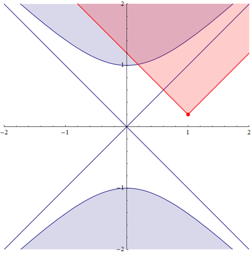
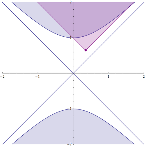
This is the so-called causality principle (or the light cone), which means, that the whole “life” of the particle in the red point is restricted by the red shaded area. How sad, isn’t it? But let’s review now a more interesting possible motion of the particle that is inside the BH horizon. As seen on the picture below (purple point and cone), the possible trajectories inside the BH are pretty restricted, as any kind of trajectory leads to the ultimate falling to the center of the BH for a finite time (finiteness of fall time simply means that the length of the trajectory is finite in terms of $$U$$-$$V$$ coordinates). So once you’re inside the black hole, you’re pretty much doomed to hit the singularity after some period of time. One should also keep in mind, that once particle moves from purple point even infinitesimally, it would then have a new ‘purple’ light cone that restricts its further motion.
Hyperbolic Tangent Transformation
Now let’s forget for a little while about our black hole, and just review a kind of coordinate transformation that we’ll require later in our analysis. Imagine an arbitrary light trajectory $$r(t)$$ in an empty space (straight line), that is characterized by a parameter $$b$$, called aiming parameter[1].
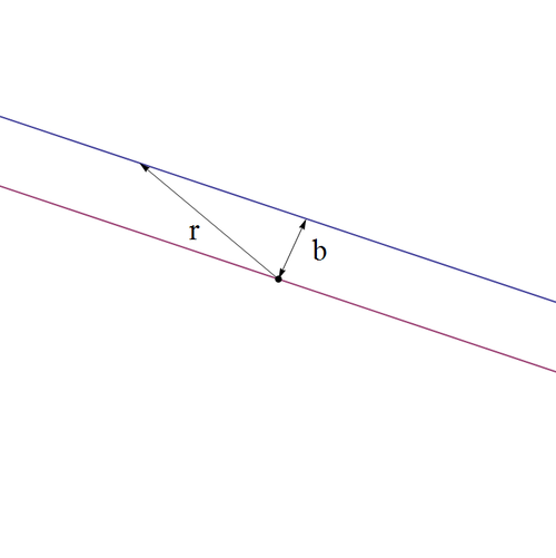
The motion of, say, photon with the speed of light along this trajectory can be represented in $$t$$-$$r$$ coordinates by the plot below. Two curves – purple and blue – represent two kinds of trajectories with $$b=0$$, and nonzero $$b$$ (here we assume that at $$t=0$$ light passes through the closest point from coordinate origin). Thus the intersection of light trajectory (‘blue’ and ‘purple’) with $$r$$ coordinate axis is the $$(b,0)$$ point. The equation of light trajectory with arbitrary $$b$$ is represented on a plot.
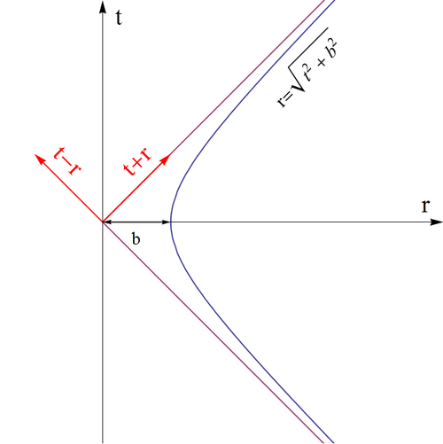
Now we want to do a coordinate transformation $$T^+=t+r$$ and $$T^-=t-r$$, the new coordinate axes are represented above in red. These new coordinates are called the lightlike coordinates, as light moves along them in 4-dimensional space (if $$b=0$$). The one bad thing for these coordinates is that we can’t really represent the infinity on our plot, thus it’s not quite convenient to use them and we want to conformally[2] transform and squeeze our infinity into something limited, hence representable on the plot. The good function we may use for this purpose is a hyperbolic tangent that transforms the $$x$$ from $$-\infty$$ to $$\infty$$, to the $$\tanh{x}$$ interval $$-1$$ to $$1$$. And for every single $$y=\tanh{x}$$ there is only one $$x=\tan^{-1}{x}$$.
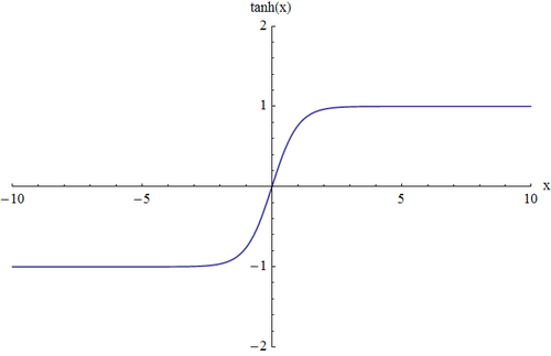
So we do a tanh transformation $$U^+=\tanh{T^+}$$ and $$U^-=\tanh{T^-}$$ (surely, we could have used an arctan transformation, that is also restricted between $$-\pi/2$$ and $$\pi/2$$, so one should keep in mind that there’s nothing special with $$\tanh$$, it’s just a function that is usually used). And now we’re happy, because in this coordinates we can visually represent the infinity on our plot.
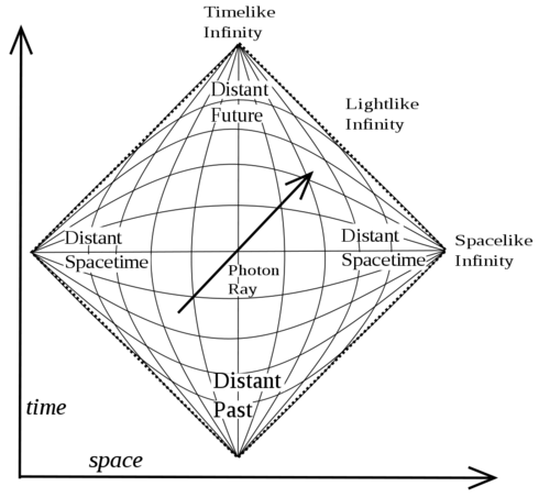
Here we have several important things to notice on our diagram. Our infinity is now smudged along the frame line having two timelike infinities and two spacelike infinities. The vertical curves on a picture represent $$r=const$$ trajectories (eternal spheres), the horizontal ones are $$t=const$$, ’spatial’ hyperspheres. So what we’ve done is we squished the spatial and time infinities into points and mapped all the infinite four-dimensional space-time into a finite region (very similar as in complex analysis we squish complex infinity which with the help of Riemann sphere). In our new coordinates, light rays come out along diagonal lines as represented below, thus we also have two lightlike infinities (‘past’ and ‘future’). This process of squeezing everything in a finite region is called “compactification”, or making a Carter-Penrose diagram.
[1] Of course this parameter has no physical meaning, as you can always put your coordinate origin wherever you wish. ↩
[2] Here ‘conformally’ just means, that for a transformation $$f(x)$$, for every $$f(x)$$ there is only one $$x=f(x)$$. ↩
cd ~